Disclaimer: The amount of information in this page will be limited since I have restrictions on how much I can share before we publish the results. Once the results are published, I’ll link the paper for more details.
The work described here was done entirely in python using LightGBM, scikit-learn, numpy, scipy and matplotlib. Initial tests were done with Tensorflow, but the ensemble Gradient Boosted Decision tree model outperformed the Multi-layer perceptron model for our data.
The idea is as follows:
SuperCDMS SNOLAB plans to use larger detectors divided into more number of channels/sections compared to previous versions of the experiment (see image below).
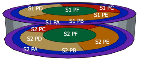 SuperCDMS detectors are partitioned into channels for efficient signal collection
The issues we are trying to address are twofold. A higher number of channels introduces increased “cross-talk” among them, resulting in undesirable correlated noise. In other words, alterations in one channel will impact others. Failure to address this issue can degrade the performance of our energy estimators.
There is a second issue we’re trying to address. Imagine you are an incoming particle going to meet your friend, the recoiling nucleus of a Ge atom in the SuperCDMS detector. You arrive at your friend’s home (the detector) but realize that your friend has just bought a bigger home. You walk to your friend and say hi. Now say the friend wants you to meet some of the guests (a signal collection mechanism) staying at his house. They call out to the guests from where they are. Because your friend’s house is now bigger, their voice takes longer to reach the guests because the sound waves now take a longer time to propagate. The guest closest to your friend’s location hears the call first, then the next one and so on. So the signals (vibrations in the crystal) are received or collected faster in channels (guest room) which are closer to the source. This is what we call ‘position dependence’ in SuperCDMS lingo. Position dependence can significantly degrade the energy resolution of our energy estimators. (the guest farthest from your friend may not hear what your friend said clearly).
The shape and height of the collected signal pulse depends on the location of the event in the detector. The height of the pulse also gives the amount of energy deposited in the crystal. SuperCDMS has developed an advanced fitting algorithm which fits multiple channels with multiple shapes or templates simultaneously to account for correlated noise, called the NxM filter. The filter itself is obtained by minimizing the following $\chi^{2}$ with respect to the vector of amplitudes, P:
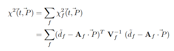
‘d’ is a vector of your data points in the time series signal. A is a matrix each of whose column is a complicated mapping of a model/template which fits the signal in frequency space, M templates each for N channels. V is a covariance matrix which captures information about the correlated noise between channels. As the name suggests, the NxM algorithm filters out signals from all the channels for each event. The output is a vector of amplitudes, P, one per channel, per template. One can interpret these amplitudes as a measure of how much each model contributes towards the shape of the signal.
Through my research, I discovered that utilizing Principal Component Analysis (PCA) allows us to create templates that capture positional information within the NxM output amplitudes. Furthermore, I found that employing machine learning techniques can address degradation stemming from positional dependence. Initially, I attempted to use a Multilayer Perceptron (MLP) with the NxM amplitudes as input and true energy as labels. However, I encountered challenges training the MLP due to limited data compared to the number of features.
I explored LightGBM for my model, given its success in other particle physics applications. Leveraging the LightGBM Gradient Boosted Decision Tree, I achieved a twofold improvement in energy resolution by correcting for positional dependence. Additionally, I successfully reconstructed event locations in the detector by training on position-labeled data.
Traditionally, we relied on position-dependent energy estimators derived from various fitting algorithms (termed Optimal Filters or OFs internally in our collaboration) or pulse rise times to establish a correlation with position in a convoluted manner. The success in reconstructing position using machine learning was particularly exciting, as it marked the first instance of relating amplitudes to physical locations on a detector. Notably, this study was conducted on simulated datasets with available position labels.
With this premise in mind, the following presentation shows a few major results: Google slides.